
Visualising Julia sets Bearbeiten
Julia sets and Fatou sets can be nice. Their computergraphical generation can be hard.
In the remainder of this page, we work out a method which can be used to visualise the Julia set of a complex function ƒ. The advantage is that you don't need to know attractors of the iteration

The generated images will be smooth in the Fatou part.
Overview: Imaging methods Bearbeiten
Note that there exist other approaches to color complex dynamical systems like
Inverse Iteration Method (IIM) Bearbeiten
Compute the preimages of ƒ, i.e. compute the reverse orbit. Because the stability of the fixed points turns from attractive to repelling and vice versa, one just choses a complex number and looks where it goes under the invers iteration. The trouble is that the results will not uniformly distributet in and that you have to compute the inverse of ƒ.

Coloring by speed of attraction (CSA) Bearbeiten
Taking a value from the lattice of points to color, perform iterations until the iterative is close to an attractor. Color the point according to the number of iterations needed to bring it close enough to the attractor.
This method is commonly used to visualize Julia sets of polynomials and Julia sets that are attached to Newton's famous method for finding the zeros of a function. Polynomials or degree > 1 always have infinity as a super-attractive fixed point. The rational function that occurs in Newton's method has always the function's roots as attractive fixed points. However, in both cases there may be other attractors, which – moreover – need not to consist of just one point.
Escape Time Algorithm (ETA) Bearbeiten
If ∞ is an attractor, i.e. a fixed point of the process, then color the point according to the number of iterations – the time – it takes until one sees the point escapes towards ∞. If the point does not escape during the maximum number of iterations, the point is colored as belonging to the Julia set or to the basin of some other attractor. This method works for polynomials. The most prominent Julia sets are the ones for z→z2+c where c is an element of the Mandelbrot set or not far away from the mandelbrot set. If you see a picture of such a Julia set, it is likely that ETA had been used to get the picture.
Cauchy Convergence Algorithm (CCA) Bearbeiten
In the remainder of this page, I will present a different approach whose idea as basically the same es that of Escape Time Algorithm. However, no basin of attraction must be known in advance and the different basins of attraction can be separated and be colored differently. The approch uses the notion of Cauchys convergence. Instead of observing the orbit of a point, this method observes how the distance of two nearby points z and z+ε evolves as these two values are iterated. If the difference tends to 0, then the point heads for an attractor. If the difference does not approach 0, then the point is close to (or a part of) the Julia set.
The Metric Bearbeiten
Let be a canonical projection of the compactified complex plane onto the Riemann sphere S2:


This gives us a metric d: As distance between two points in the complex plane we take their distance on the sphere, i.e. the length of the orthodrome. This means that the metric is bounded by π and even the distance to ∞ (which is now the north pole) is finite.
In order to compute the distance between two points z and w we rotate the sphere S2 in such a way that
- w maps to 0
- z maps to the positive real axis
After these transformations the distance can be computed quite easily. The rotation can be accomplished by a squence of isometric Möbius transformations. All an all, we get

which is left as an exercise to the reader. The bar denotes complex conjugation. The metric is then

The nice feature that is introduced by d is that sequences that formerly diverged against infinity now converge towards infinity, i.e. towards the north pole of S2.
Stability of Orbits Bearbeiten
Recall the definition of the Julia set for a contraction mapping ƒ. The definition implies some facts on the stability of the iteration

where ƒn denotes the n-th iterative of ƒ:

The set

is called Orbit of z (under ƒ).
The orbits of two points z and w behave similar − in some sense − if z and w lie close together and belong to the Fatou set Fƒ which is the complement of the Julia set Jƒ of ƒ. If z is an element of Jƒ then z and w will behave quite different, even if w itself is an element of Jƒ.
To get a notion of the stability of an orbit, we set

for a small ε and with the metric d from above. This means that we take two points which are close together, and then we summarize their distances as ƒ makes them jump around on the Riemann sphere. Note that for any fixed ε the sum can diverge for large n even if z is a Fatou point.
However, we can use Σn to measure how close a point is to Jƒ: the larger the sum is, the more instable is the iteration and the closer is the point to the Julia set of ƒ.
To destinguish points of (or close to) the Julia set from points in the Fatou set, we need a creterion. To get it, we compute all the Σ-values for the points that we want to color, i.e. for all points in a lattice Γ. After computing these values, we do a little bit of statistics to get the expected value E and the standard deviation σ for the set of Σ-values: Let

Remind that

It turns out that the values Σ are widely spread over several scales. Therefore, we do not use Σ directly. Instead, we use the logarithm of Σ. The value δ is just a small constant to avoid the logarithm's input to be zero.
Coloring Bearbeiten
Now, we have all we need to color a point:
- choose
- a lattice of points to color
- the number of iterations to perform
- a small
- for all points, compute
- compute and
- compute


for some constant . Because will be used to separate points that belong to the Julia set ( ) from points that to not ( ), reasonable values for are greater than . Try settings like or or the like. If then we color as belonging to the Julia set. If we can use that value to shade the Fatou set. If we know some attractor, we can check if ƒ is close to it and use that information, too.


To map values to the valid ranges for saturation and brightness we use the function from section helper function h.

Modifications Bearbeiten
The computation of takes a lot of time. The visualisation process needs two passes:
- compute from all
- color the points using and recomputed

Alternatively
- compute and store all
- compute and color the points
An other approach looks like that:
- Find the smallest so that is below a given bound for all . If no such can be found, then assume to be an element of the Julia set. Otherwise, use to color the Fatou set.


This algorithm is a variant of the escape time algorithm (ETA). Note that in ETA the point does not really escape (at least if we are on the sphere), it just converges to ∞. This approach is similar. However, we don't need to know an attractive fixed point of ƒ.
Up to now, I didn't try the modified version. One disadvantage may be that the Fatou set will no more appear smooth colored. Then I am not sure if this modification is really an advantage, because the iteration must be done until a given maximum number of iterations is reached. Note that even if is under the bound for some the distance can rise again. I cannot say if this effect is crucial or can be neglected...


Gallery Bearbeiten


denotes the Newton operator


Using Critical Points Absorption (CPA) Bearbeiten
The previous method yeilds neat, smooth colorings and requires least knowledge about the dynamics of the process. However, it is quite time consuming. Teh following approach is an extension of escape time algorithm (ETA) for polynomials.
Let ƒ be a polynomial of degree d > 1 over C. Such a polynomial has at most d critical points: infinity and the at most d–1 zeroes of ƒ′. It is well known that each attractor of the process z→ƒ(z) absorbs at least one critical point. Suppose zK is a critical value, then ƒn(zK) comes arbitrarirly close to one of the attractive cycles of ƒ.
A process for a quadratic polynomial ƒ(z) = z2 + c is the simplest case: The critical values are 0 and ∞. As ∞ absorbs itself, only 0 is left, and we have the following cases. M denotes the Mandelbrot set.
- Easy case. 0 is absorbed by ∞, and J(ƒ) consists just of Cantor dust. Escape time to ∞ can be used to color all points.

- If c is an element of the interior of M, then 0 will be absorbed by a (super) attractive cycle. Compute
- for a sufficiently large n. As w (basically) only depends on c, it can be precomputed before starting the visualization of J(ƒ). Notice that w is the element of a cycle that might have more than one element, i.e. w is only unique modulo that cycle.


- Coloring for a point z in C is then as easy as ETA:
- If z is absorbed by ∞, use escape time to color z.
- If ƒn(z) comes close to w, i.e if |ƒn(z) – w| < ε for the first time, use that n to color z.
- If ƒn(z) neither comes close to ∞ nor comes close to w, then color z as part of J(ƒ). Only few z will fall into this category.
Visualising complex functions Bearbeiten

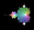
Suppose we want to visualise a complex valued function like

In order to color we decompose it into its absolute value and its argument .


Then, we assign the color

to the point representing . In this HSV color space, all values are in the range from 0 to 1. The first component (hue) of the HSV color depends only on the argument of and the second and third component (saturation and value) depend only on the absolute value of . We use a transformation on to map it into the interval . For see section helper functions.

![{\displaystyle [0,1]}](https://wikimedia.org/api/rest_v1/media/math/render/svg/738f7d23bb2d9642bab520020873cccbef49768d)

Examples Bearbeiten
The values indexed s (saturation) control the transition saturated colors→white (resp. gray scale), i.e. intermediate values → infinity. The values indexed h (value/valenz) control the transition black→bright, i.e. zero→nonzero. Parameter a controls where the transition takes place: a is just the radius of the circle dividing the two regions (dark/bright, saturated/gray, etc.) Parameter b controls how sharp the transition is: b small = soft, b large = sharp.
The following images all show the range [-10,10]×[-10,10] and use (radius of rainbow) and (radius of black disc).


In the image with swapped meanings of S and V zero is printed in white and infinity in black.
Gallery Bearbeiten
- Some examples of colorings
-

-

-

-

Roles of S and V interchanged


- Analysis of critical point of z→z²+c
-
 n=1: starting values (color map)
 -
 n=2
n=2 -
 n=3
n=3 -
 n=4
n=4 -
 n=17
n=17 -
 n=18
n=18 -
 n=19
n=19 -
 n=20
n=20


Helper functions Bearbeiten
Helper function t Bearbeiten
.svg)

is a smooth, monotone sigmoidal transition from −1 to 1 that satisfies and . There are many choices for it. Some of them are


with gd denoting the gudermannian function.
- All functions in a Desmos plot.
Helper function h Bearbeiten
.png)

Helper function is almost the same like but it maps to and we can adjust the speed of transition by parameter .


with . Then is symmetric to the point (0, 1/2) and


Negative values are mapped to values between 0 and 1/2. Positive values are mapped to values between 1/2 and 1. The parameter controls how fast the transition will be.
If we want a falling function, we can use the symmetry

i.e. we negate or .

Helper function g Bearbeiten
.png)

This function maps the positive numbers to the interval .


for some function that is defined below. If is appropriately chosen then for the following holds


This means that
- grows continuously from 0 to 1 as grows from to
- we can control where crosses the middle between 0 and 1 by specifying parameter
- we can control how fast passes the point by specifying parameter


We are left with determining the finction on with

.png)

must satisty

For we set

Helper function w Bearbeiten
.png)

This function maps the positive numbers to the interval .

By we can control its slope in the origin:

Circular arc through (0,0) and (1,1) Bearbeiten
A circular arc through (0,0) and (1,1) that has given slope of in (0,0) and in (1,1):


where

The center of the circle is incident on the line .

Bézier-Curves Bearbeiten
Quadratic Bearbeiten
Suppose we have a smooth function
![{\displaystyle {\begin{aligned}f:[t_{0},t_{1}]&\;\to \;\mathbb {R} ^{2}\\t&\;\mapsto \;(x(t),\,y(t))\\\end{aligned}}}](https://wikimedia.org/api/rest_v1/media/math/render/svg/1d92426221ea22947ad5b9f43715c38d02b8487c)
and like to draw an approximation of it using quadratic Béziers. Obviously, the two end points lie on ƒ and the control point lies on the crosspoint — for simplicity, we assume it exists — of the two tangents through the bounding points. In other words, we have to determine the intersection of the two lines

with canonical abbreviations like

This leads to a determining equation for the λ's

whose solution is

This gives us the intersection, i.e. the control point, by evaluating one of (or the two of) the g's at the end point(s).
Cubic Bearbeiten
Desmos: Interactive, cubic Bézier
Suppose we have a smooth function
and like to draw an approximation of it using cubic Béziers

From the two last representations we see immediately the value of the derivatives of b in the end points. We want the first and second derivatives in the end points to point in the same direction as the derivatives of ƒ do. Thus

We get the coordinates (1, 1/2) and (1/2, 1) for the control points (red). The resulting bézier (orange) does not approximate the circle as good as possible.

and together with ƒ0=P0 and ƒ1=P3 we get the linear system

Note that in the special case of x(t) = t we get

i.e. the x-coordinates of the control points P1 and P2 divide the interval [t0,t1] with ratios 1:2 resp. 2:1. This is quite astonishing because in order to get the control points we do not have to evaluate second derivatives of ƒ. This is due to properties of Bernstein polynomials.
To solve the above system we use standard technique like the adjugate.
Also note that if both second derivatives of x or both second derivatives of y happen to vanish the above system won't have full rank, i.e. the corresponding matrix won't be invertible. However, it's sufficient to determine α and β to get the control points and for vanishing second derivatives we get the less complicated systems

resp.

Solving this yields

and ditto for y.
As you can see in the image above, there is some room for improvement and therefore we work out a second approach. Again, we set P0=ƒ0, P3=ƒ1 and constrain the two control points P1 resp. P2 to lie on the tangent through the end point next to it. This leaves us again with a two dimensional space to search in. Instead of imposing properties on second derivative, we now simply force the bézier to meet the curve ƒ in a third point Q, i.e. we set
![{\displaystyle Q=f_{t}=f(t\cdot t_{0}+(1-t)\cdot t_{1})\quad {\stackrel {.}{=}}\quad b_{[P_{0},P_{1},P_{2},P_{3}]}(t)}](https://wikimedia.org/api/rest_v1/media/math/render/svg/5092cec809d87502ab9a3f0b84b9df1554fd5edf)
for some t in (0,1) and b denoting the bézier. The condition on the end and control points again reads as

We get the coordinates (1, ω) and (ω, 1) for the control points (red) with

The resulting bézier approximation (orange) is fine. There is no visual difference between the circle and the bézier. The additional point Q is indicated halfway on the bow.

Putting this together with the condition on Q we get

Note that we can use more than one point Q. Suppose we like to use n points Qi to guide the bézier. Each Qi will add two more lines in the above linear system, i.e. the system will look like

with a 2n-dimensional vector w and a 2n×2 matrix M. In general, this system is overdetermined and thus has no solution. Therefore, we solve the 2-dimensional system

instead which yields a least-square solution for α and β.
We make the above system a little bit more explicit for the case of one additional point at t = 1/2. The linear system then reduces to

Note that the same matrix already occured in the computation for quadratic bézier curves above, however the matrix now gets multiplied with a vector describing the curvature, whereas in the quadratic case it gets multiplied with a vector descriping the direction.
If the special case of a linear function x we get

noname Bearbeiten
Suppose we have a smooth function
![{\displaystyle {\begin{aligned}f:[t_{0},t_{3}]&\;\to \;\mathbb {R} ^{2}\\t&\;\mapsto \;(x(t),\,y(t))\\\end{aligned}}}](https://wikimedia.org/api/rest_v1/media/math/render/svg/886f6bddf5ef94dc5a4b7b21f2e517d02d57c1bf)
from the reals to the plane and like to draw an approximation of it using cubic Béziers.
Let u be a second function with fixed points at t0 and t3 which is smooth and monotone. Then the composition ƒ o u will yield exactly the same plot for any such u. Applying function u means that drawing the curve at different, arbitrarily increasing and descreasing speeds does not change the way the plot of the curve looks like. That is nice from the plotter's point of view. However, this generates some difficulties when we try to approximate the curve, which eventially turns out to be a playing field for calculus of variations that will lead to formulas and partial differential equations much too complex for practical considerations. So we look for some characteristics that are invariant under reparameterisations u.
The derivative of ƒ o u is the velocity[1]

This furmula is the rationale why the first derivative of the bézier curve shall point in the same direction as the first derivative of ƒ: the direction is independent of the parametrisation u. The speed v always points into the same direction, no matter how fast we drive along ƒ. This is no more true for the acceleration

In the remainder of the essay we will only use properties of the curve at its end points. Thus, before we proceed, let's use the fact that u has fixed points in the t-valueas that yield the end points in order so simplify the formulas for v and . The formulas then read

provided we evaluate these quandities at one of the end points.
We can think of as being composed of two orthogonal components: one in direction of motion that speeds up or slows down the pencil, and on perpendicular to v which leads to a change in direction. The projection of onto the direction normal to v is parallel to[2]


Sphärengleiche Linear Transforms Bearbeiten
Given a linear transfrom in n-dimensional euklidean Space:

We call two linear transforms A and B spärengleich if they map the unit sphere to the same set:

Obviously, this ~ is an equivalence relation and we look for a representant of each equivalence class. We observe that this relation preserves the spectral norm

and that orthogonal matrices don't change the equivalence class:

for any A. The last line is immediately clear because orthogonal transformations map spheres to themselves. The preservation of spectral norm follows from the definition of spectral norm. Let

be the singular value decomposition (svd) of A. Then we have

and

However, the converse is not true.
Arcsin Bearbeiten


In order to approximate arcsin and arccos if the argument is close to 1 the following expansions might be useful:

with a rational power series

where !! denotes the double factorial. The radius of convergence of a is 2. We start by observing that

which can easily verified by differentiaton. It follows that

Also note the following half-argument relations for –2 ≤ x ≤ 2:

N-th derivative Bearbeiten

Again, !! denotes the double factorial. Note that for k < 0, k!! = 1.
Approximation of arcsin and arccos Bearbeiten


![{\displaystyle [0,1/2]}](https://wikimedia.org/api/rest_v1/media/math/render/svg/bf40737bcb67d2b44e2827874fcbbc9e9d133ee1)


![{\displaystyle [1/2,1]}](https://wikimedia.org/api/rest_v1/media/math/render/svg/dbd8343b09495a17d415b591ad5e3f8b0290b766)
For 64-bit IEEE double computation (53-bit mantissa) of arcsin and arccos we use the following approach:
- If 1/2 ≤ |x| ≤ 1, compute

- If |x| ≤ 1/2, compute

We have to evaluate a(x) for x in [0, 1/2] and use the following rational MiniMax approximation of order [5/4] with a relative error below 6·10−18:

with
p(x) =
+ 0.99999999999999999442491073135027586203
- 1.0352340338921976278427312087167692142 x
+ 0.35290206232981519813422591897720574012 x^2
- 0.043334831706416857056123518013656946650 x^3
+ 0.0012557428614630796315205218507940285622 x^4
+ 0.0000084705471128435769021718764878041684288 x^5
q(x) =
+ 1
- 1.1185673672255329236623716486696411533 x
+ 0.42736600959872448854098334016758333519 x^2
- 0.063555884849631716599421483898013782858 x^3
+ 0.0028820878185134035637440105959294542908 x^4
(Note: A [4/5] rational MiniMax is even better, the relative error stays below 4.9·10−18.)
Then we use the symmetries


of arcsin and arccos to get the desired result(s) over all of .
![{\displaystyle [-1,1]}](https://wikimedia.org/api/rest_v1/media/math/render/svg/51e3b7f14a6f70e614728c583409a0b9a8b9de01)
In order to achieve IEEE single precision, we can use

over with a relative error below 2.6·10−9.
![{\displaystyle [0,0.501]}](https://wikimedia.org/api/rest_v1/media/math/render/svg/63fd7cd28c115f2f132d7b4cdee2cbdd9af62056)
The relative error for arccos stays below 2.6·10−9, whereas the one for arcsin stays below 5·10−9. See a Desmos plot of the relative errors.
Error Analysis Bearbeiten
Using functional equations to get arcsin and arccos for all values in makes the relative error more complicated than usual. Let denote the relative error of at 0. Then we get the following envelopes for the relative errors (up to sign):


Some special values −1 −0.5− −0.5+ 0 0.5− 0.5+ 1 0 2 1 1 1 2 0 2 0 0.5 0.25 0 0.5 1 1 1
![{\displaystyle \max([-1,1])}](https://wikimedia.org/api/rest_v1/media/math/render/svg/06f5b46748268ea5e8c14233e3605e04ce5647f1)


Moduli Space of plane Triangles Bearbeiten
Moduli space of similar, plane triangles is again a triangle (kind of).
Dobble Spot It Bearbeiten
Dobble is a card game to have a nice time with fast pattern recognition. Each card shows 8 different icons, and any two cards have exactly one icon in common. The task is to find this common icon as fast as possible.
This essay is about how such a deck of cards can be constructed, and it supplies some mathematical background. As Dobble is famous for that mathematical background, we won't get too much into the theory; many articles found on the net address that background. A deck of card consists of 55 cards, each showing 8 different icons out of a set of 57 icons. So how do we have to arrange these icons on the cards so that any two cards picked at random have exactly one icon in common?
The property
- any two cards have exactly one icon in common
reminds of a theorem in plane geometry:
- any two different lines in the plane meet in exactly one point
Well, almost. In Euclidean geometry there are lines in the plane that don't meet, namely parallel lines. Before we go into details, let's summarize the geometric objects and how to associate to them a deck of cards, and how properties of the game arise from properties in geometry.
The two different Ways to identify Objects of Dobble with Objects in Geometry Projective Plane
of Order QDeck of Cards
Cards = Lines, Icons = PointsDeck of Cards
Cards = Points, Icons = LinesQ2+Q+1 Lines Q2+Q+1 Cards Q2+Q+1 Icons Q2+Q+1 Points Q2+Q+1 Icons Q2+Q+1 Cards Each line passes through Q+1 points Each card shows Q+1 icons Each icon is shown on Q+1 cards Each point is incident on Q+1 lines Each icon is shown on Q+1 cards Each card shows Q+1 icons Any two different lines meet in exactly one point Any two different cards have exactly one icon in common Any two different icons are shown together on exactly one card Any two different points uniquely determine one line Any two different icons are shown together on exactly one card Any two different cards have exactly one icon in common
- Properties of Dobble
- Dual properties which do only apply to a complete deck of Dobble with 57 cards. As mentioned below however, Dobble in incomplete as it comes with 55 cards only. Therefore, the dual properties do not hold for the Dobble you can buy.
In order to overcome the problem with parallel lines in Euclidean geometry, we switch to projective geometry which doen't come with that shortcoming. Whereas points in the Euclidean plane can be regarded as pairs of numbers (x,y), points in the projective plane are triples (x : y : z) such that not all three are equal to zero. In addition, we consider two triples P and P' as the same if they are multiples of each other, i.e. if there is a number λ ≠ 0 such that

A line g in the projective plane is given by a triple (gx : gy : gz) and a point P = (x : y : z) is incident on the line provided

This is similar to the Euclidean case where a point is incident on a line if

but in projective space the additional symmetry in the formulae for the point-on-a-line relation has its counterpart in the additional symmetry of any two distinct lines meet in exactly one point. Notice that if z ≠ 0 we can divide the projective condition by z, and the outcome is basically the condition for Euclidean space. However, in the projective case there are also points with z = 0 which don't have a counterpart in Euclidean geometry. These points are sometimes called the horizon or points at infinity, but we don't need such fuzzy wording or any distinction of different classes of points to construct a deck of Dobble.
The second difference to ordinary geometry is that a deck of cards consists only of finitely many items: a finite number of icons, a finite number of cards, and a finite number of icons per card. This is handled by considering geometry over a finite field instead of geometry over the Reals. A field is an entity which features addition and multiplication, both commutative and connected by the distributive law. The addition of any element can be undone, and the element that doesn't change the result of an addition is called zero and denoted as 0. The multiplication with any element except 0 can be undone, and the element that doesn't change the result of a multiplication is called one and denoted as 1.
So let's switch to a finite field F with Q elements. The first observation is that there are only finitely many points in the plane. There are Q3 triples of the form (x : y : z) with x, y and z in F. As not all three coordinates shall be zero, we are left with Q3−1 non-zero triples. Triples which are a multiple of each other are regarded as the same point, and because there are Q−1 non-zero values in F which can serve as the factor λ from above, we get the total number of points of the projective plane over the finite field F of order Q as

This is also the number of lines in that plane because the lines are also represented as triples. In order to see how many points are incident on each line, let's enumerate the points as

If the x-coordinate is non-zero, we can divide all coordinates by x which gets us the points of the form (1 : y : z). If x is zero and y is non-zero, then divide by y to get the points of the form (0 : 1 : z). If both x and y are zero, that point can be represented as (0 : 0 : 1) because z must be non-zero then.
In order to compute which points are incident on which line, we could just do brute force and iterate over all lines and all points and test whether or not the relation from above is satisfied. But we can do better by working out explicit formulae. To that end we use a different relation to determine whether a point is incident on a line:

This is just a rearrangement of points which does not change the global structure. The advantage is that in our enumeration of points and lines, the first coordinates, i.e. x and gx, are always 0 or 1 which will simplify the computation.
Lines and Points incident on it Line g = (gx : gy : gz) Constraint(s) on
coordinates of PP = (x : y : z) Case (1) (2) (3)


In either case, there are Q+1 points on each line, and it's easy to verify that any two distinct lines have exactly one point in common. Due to the duality of points and lines, each point is incident on Q+1 different lines.
The case Q = 2: Fano Plane Bearbeiten

| (0:0:1) | ||
| (0:1:0) | ||
| (0:1:1) | ||
| (1:0:0) | ||
| (1:0:1) | ||
| (1:1:0) | ||
| (1:1:1) |

Let's work out the simplest case of Q = 2, the Fano plane. The field F is the Galois Field GF(2), the field with the 2 elements 0 and 1. We expect 22+2+1 = 7 lines and hence also 7 points, each line passing through 2+1 = 3 points, and each point incident on 3 lines.
| Case | Line | Points | Cards | ||||
|---|---|---|---|---|---|---|---|
| (1) | (0:0:1) | (0:0:1), (0:1:0), (0:1:1) |
| ||||
| (2) | (0:1:0) | (0:0:1), (1:0:0), (1:0:1) |
| ||||
| (0:1:1) | (0:0:1), (1:1:0), (1:1:1) |
| |||||
| (3) | (1:0:0) | (0:1:0), (1:0:0), (1:1:0) |
| ||||
| (1:0:1) | (0:1:0), (1:0:1), (1:1:1) |
| |||||
| (1:1:0) | (0:1:1), (1:0:0), (1:1:1) |
| |||||
| (1:1:1) | (0:1:1), (1:0:1), (1:1:0) |
|
The case Q = 7: Dobble Bearbeiten
For Q = 7 we get Dobble: 57 icons on 57 cards, each card displaying 8 icons. But wait — a deck of Dobble consists only of 55 cards, not of 72+7+1 = 57. Why that? Nobody knows! Two cards are "missing" and not contained in the game. These two missing cards would show the following combinations of icons:
- snowman, exclamation mark, dog, eye, light bulb, ladybug, skull, hammer
- snowman, question mark, gingerbread man, maple leaf, cactus, daisy, ice cube, dino
Due to these two missing cards, some of the statements won't hold for Dobble: For example, not all icons are present 8-fold in the entire game. In particular, the snowman is only present 6 times as it is the icon common to the two missing cards. And not for any combination of two icons there is a card showing that combination. For example, there is no card showing both dog and eye because this combination belongs to one of the missing cards.
Beyond Dobble Bearbeiten
A central object in the construction from above is the field F which only exists if Q is the power of a prime number p, i.e. Q =pn for some prime number p and a natural number n ≥ 1. What happens if Q is not the power of a prime? We can use a rather axiomatic approach and define the projective plane of order Q to be an entity consisting of Q2+Q+1 points, Q2+Q+1 lines, each line passing through Q+1 points, each point incident on Q+1 lines, any two points uniquely determining a line, and any two lines having exactly one point in common.
For Q = 1, the construction from above still works provided we take the "1" in the formulae literally and set the free variable (z in cases (1) and (2), y in case (3)) to 0. That yields a game with 3 cards, each showing 2 icons out of a set of 3 icons. This works even though there is no field with one element.
For Q > 1, the Bruck–Ryser theorem adds some constraints on Q: If a projective plane of order Q exists and Q is 1 or 2 mod 4, then Q must be the sum of two squares. Hence, if Q is 1 or 2 mod 4 but not the sum of two squares, e.g. Q = 6, then no projective plane of order Q exists. However, there are infinitely many numbers remaining to which the theorem does not apply, the first one being 10 — the only case where an answer is known so far. The result for 10 has been achieved by heavy computation. The next greater value which is not the power of a prime and where the Bruck–Ryser theorem does not apply is Q = 12 with 13 icons per card and 157 cards. Taking a pure combinatorial approach we get

different 13-icon subsets (possible cards) which can be built out of the 157 icons, and for a complete game we have to pick 157 from these 3.3·1018 cards in such a way that all the axioms are satisfied.
Linear Recurrence Bearbeiten
Suppose the linear recurrence

for where , ..., are given numbers.


We want to determine an explicit representation of . To that end, write the recurrence as:


so that it takes the form

Now suppose has different eigenvectors and we know all of them, including the corresponding eigenvalues . Then we can write:


where the are scalars in the algebraic closure of and is a matrix with the eigenvectors of as columns. Hence:


which leaves is with the computation of the , the and the . Once we determined the eigenvectors, we get the by means of:

Expanding the determinant of by expanding after it's top row, we find that all eigenvalues satisfy the characteristic equation


From this we easily see that the eigenvectors of are:

Due to (1), in order to get we take the top component of to get:


Thus we are finished: Depending on the , the eigenvalues can be computed explicitly or by numerical methods. From the eigenvalues we get the matrix which we use to compute the coefficients from the starting values ... so that we have determines all unknowns in (2).

Example 1 Bearbeiten
Let so that we get the Fibonacci sequence


with the characteristic equation

Finding solutions of ln cosh x = αx + β Bearbeiten
The graph of

is convex and loosely resembles a hyperbola

In particular, for large . The convexity of allows for easy specification of the number of solutions of


(1)
| ||

If the line is tangent to , then there is a uniqe solution of multiplicity two. If then (1) has a unique solution, and for the number of solutions depend on whether the line runs below a tangent to or above:


with

and where stand for "one solution of multiplicity two".

The procedure to approximate solutions of (1) is then as follows:
- Compute , the number of solutions of (1). If , then terminate with "no solution".
-
Compute the solutions of
(2)
for . The hyperbola has the property that (2) has at least as many solutions like (1) has. If but (2) has two solutions and , then use . The solutions of (2) are the solutions of
where
This is a quadratic equation in , except when where it is linear with solution . In the quadratic case, the number of solutions are 0, 1 or 2, depending on whether the discriminant satisfies , or , respectively:
- We determined approximate solutions in step 2. For each initial approximation ,
perform Newton-Raphson iterations for (1) until the desired accuracy is reached:


Finding solutions of ax + bx = c Bearbeiten
For we want to determine approximate solutions of


(1)
| ||

Before handling the general case, sort out the special case :

- If , then there is a single solution .


- If , we can take any , and if , then there are no solutions.


In the general case of , transform to the equivalent problem

(2)
| ||

handled in the previous section, where

The solutions of (1) are then given by

where ranges over all solutions of (2).
Finding solutions of ax − bx = c Bearbeiten
For , we want to determine approximate solutions of


(1)
| ||

If , then the solution is , except when which allows any .

If , then we solve the equivalent problem with . Thus, without loss of generality, we may assume in the remainder.


Before treating the general case, sort out the special cases and :

- If , then there is no restriction on if , and if there is no solution.

- If , then the solution is .


In order to solve the general case , transform to the equivalent problem

(2)
| ||
handled in a previous section, where

The solutions of (1) are then given by

where ranges over all solutions of (2).
Finding solutions of ax + bx = cx Bearbeiten
For we want to determine approximate solutions of
(1)
| ||

- If or , then there is no solution.


- If , then the solution is .


In order to solve the general case, transform to the equivalent problem
(2)
| ||
handled in a previous section, where

The solutions of (1) are then given by

where ranges over all solutions of (2).
Finding solutions of xr = ax + b Bearbeiten
For we want to determine approximate solutions of

(1)
| ||

Split the problem into several special cases. Once a special case has been treated, the assumption is that it won't occur in the cases below.
- r = 0
-
- : All possible are solutions if . If , there are no solutions.
- : The solution is .
- r = 1
-
- : All possible are solutions if . If , there are no solutions.
- : The solution is .
- r < 0
-
Solve the equivalent problem
(2)
where , a case handled below. Solutions of (1) are then of the form , where iterates over all non-zero solutions of (2).


In the remainnder, we will have to consider three different kinds of exponents :

- Odd exponents: The exponent has a representation where and are odd integers.
- Even exponents: The exponent has a representation where is an even integer and is an odd integer.
- Real exponents: The exponent neither fits the odd case nore the even case.


- a = 0
-
The solutions of (1) are the solutions of
(3)
which are:
(4) - 0 < r < 1
-
Set and solve the problem
(5)
with . Solutions of (1) are then where iterates over all solutions of (5). If is not odd, then the solutions must satisfy .
In addition, for even exponents there are solutions that satisfy , where ranges over solutions of
(6) - r > 1
-
All other cases have been reduced to this one (or have been handled as special cases).
Noice that we have .
In order to simplify this presentation, assume that we only have odd and even exponents.
The real case is mapped to the even case by assuming
(7)
is an even function. After we computed all solutions, we ditch negative solutions if the came from the real case.


